[Tutorial] Principal Component Analysis

In data science, Principal Component Analysis (PCA) is a popular technique to reduce the dimension of a dataset. Picture this: data can sometimes be overwhelming with its many dimensions, much like a city with a lot of streets and alleys. In this analogy, PCA doesn't just show us every winding alley – it points us to the main roads and iconic landmarks.

In a more technical term, PCA transforms the data into a set of new variables known as principal components. Each of these components is ranked based on its significance, meaning the most impactful ones capture the majority of the data's variance. As a result, patterns, trends, and outliers become more evident or even discovered in the reduced data; therefore, one can simply focus on these main components.

Principal Component Analysis

The primary objective of PCA is to reduce the complexity of data while preserving as much information as possible. So, instead of dealing with, let's say, 100 different factors, we can just look at the main 2 or 3 that capture most of the story. A simple analogy can be found when recognizing a face: "I know that all faces have similar structures, but this uniqueness of nose and eyebrow combo is John's, for sure!"

The concepts and derivations presented in the following are inspired by and adapted from a session on Principal Component Analysis that I attended in 2022, delivered by Prof. Baoyuan Wu. Any interpretations, extensions, or errors are my own.

There are two objectives for PCA that we are after. First, when reducing the dimension of a dataset, we want to make variance as large as possible. This concept is to spread the data points as widely as possible while keeping their relative positions to each other, pertaining its similarity when reduced. Second, we want to make the reconstruction error as minimum as possible, making sure that we don't lose too much original information. Both ideas' derivation are shown below.

Derivation by Maximal Variance

As an conceptual overview, let's first understand the main reason of having the variance to be maximal. For instance, what does it mean to maximize it?

When we are reducing the dimensions of data using PCA, we are essentially trying to condense the information. By maximizing variance, we ensure that we are focusing on the most crucial patterns or structures in the data. By focusing on high variance, PCA gives us a summary of our data.

Suppose we have a dataset

D={d1​,d2​,…,dn​}∈RN and we want to map it into a $K$-dimensional subspace $S$ such that the variance of reconstructions is maximal, i.e.,

, where

μ˜​=n1​∑i=1n​d˜i​ and ${\tilde{d}}_i\in \tilde{D},\forall i\in \{1,2,\dots ,n\}$, $\tilde{D}$ is the new projected dataset. Of course, the projected $d_i$, ${\tilde{d}}_i=(\frac{1}{n}{\sum }_{i=1}^n{d}_i)+{\text{Proj}}_S(d_i-\mu )$, is spanned by an orthonormal basis $U=\{u_i{\}}_{i=1}^K$ where:

• $u_i\in {\mathbb{R}}^N$,
• $\parallel u_i\parallel =1,\forall i$, and
• $u_i^T{u}_j=0,i\ne j,\forall i,j$

Denote

μ=n1​∑i=1n​. Then,

This implies that:

Derivation by Minimal Reconstruction Error

Again, as an conceptual overview, let's first understand the main reason of having the reconstruction error to be minimal.

When we project our data onto a lower-dimensional subspace, we are essentially compressing the data, resulting in some information loss. The reconstruction error measures this loss: the difference between the original data and the data reconstructed from its lower-dimensional representation. Ideally, we want this error to be as small as possible, implying our compressed representation is a good approximation of the original data.

By definition, our objective is

Equivalence of Both Derivations

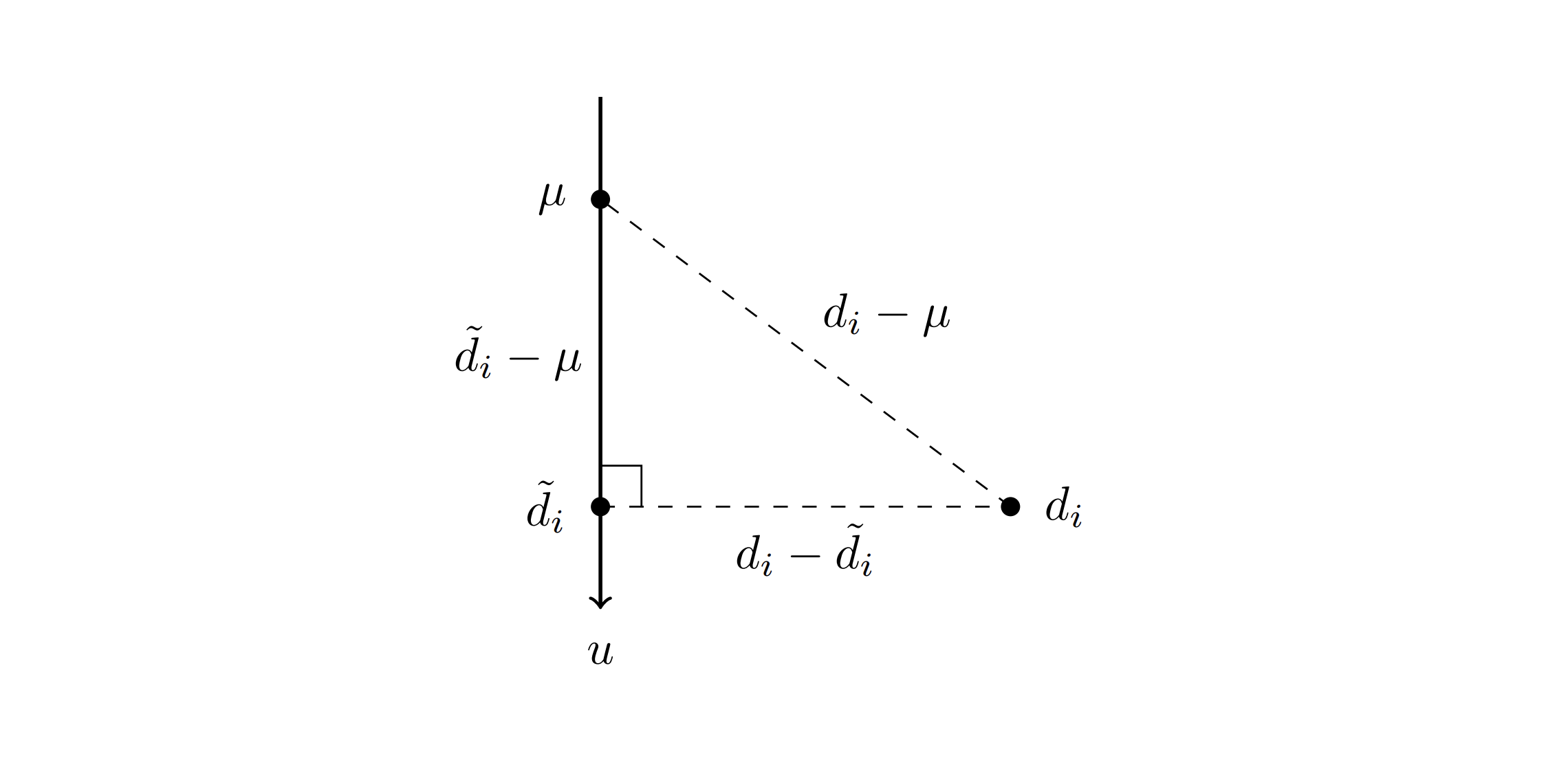
By Pythagorean Theorem,

Since

n1​∑in​∥di​−μ∥2 is a constant, we conclude that the objectives of both derivations are equivalent.

Lagrange Function Formulation

I touched upon Lagrange Relaxation in a previous blog post, which you can find here. If this topic interests you, I recommend starting there for some foundational understanding.

, where

Σ=n1​∑i=1n​(di​−μ)(di​−μ)T. The formulation of our optimization problem to a Lagrange function is as follows:

, where

Λ=diag(Λ1​,Λ2​,…,ΛK​). Then, the optimal solution satisfies:

Singular Value Decomposition

If you are unfamiliar with Singular Value Decomposition, I recommend referring to some resources, one of which is this very blog.

The previous suggests that the optimal solution

ui​ must be one of the eigenvectors of $\Sigma$. We can then perform Singular Value Decomposition on $U^T\Sigma U$, as demonstrated below:

, where

λ(i)​ denotes the $i$-th largest value in $\{{\lambda }_1,{\lambda }_2,\dots ,{\lambda }_n\}$.

Implementation

import numpy as np
from numpy.linalg import eig

def PCA(D, K):
    n = len(D)
    D = np.transpose(np.array(D))

    mu = np.mean(D, axis = 1)[:, None]
    D_mu = D - mu

    # Calculate empirical covariance matrix
    empirical_covariance = np.dot(D_mu, np.transpose(D_mu)) / n

    # Perform SVD decomposition for empirical covariance matrix
    eigenvalues, eigenvectors = eig(empirical_covariance)

    # Take the top K eigenvectors
    sorted_indices = np.argsort(eigenvalues)[::-1]
    U = eigenvectors[:, sorted_indices[:K]]

    return np.transpose(np.matmul(np.transpose(U), D - mu)).tolist()

D = [
    [-1, 2, -3],
    [2, 0, -1],
    [1, 1, 1],
    [-1, -2, 0],
    [2, 1, 3],
    [0, -1, 2],
    [-2, 1, -1],
    [1, -2, 2],
    [3, 0, -2],
    [0, 1, 1]
]
print(PCA(D, 1))

Closing

We have seen Principal Component Analysis' ability to simplify complex data. By focusing on what's essential and reducing unnecessary noise, PCA provides a clearer perspective on the underlying patterns in our data. It's a key tool in data science, but it's important to use it wisely, ensuring we don't overlook critical details in our simplicity quest.

References

1. Baoyuan Wu, "Principal Component Analysis," The Chinese University of Hong Kong, Shenzhen, 2022.
2. Hervé Abdi, Lynne J. Williams, "Principal component analysis," Wiley Interdisciplinary Reviews: Computational Statistics, 2010. https://doi.org/10.1002/wics.101.

© 2023 Yohandi. All rights reserved.